 MathCS.org - Statistics
back | next
6.1 Correlation between Variables
In the previous section we saw how to create crosstabs tables, relating one variable with another, and we computed the Chi-Square statistics to tell us if the variables are independent or not. While this type of analysis is very useful for categorical data, for numerical data the resulting tables would (usually) be too big to be useful. Therefore we need to learn different methods for dealing with numerical variables to decide whether two such variables are related. In addition, the new techniques will allow us to make predictions of future events based on events in the past.
Example: Suppose that 5 students were asked their high school GPA and their College GPA, with the answers as follows:
Student HS GPA College GPA A 3.8 2.8 B 3.1 2.2 C 4.0 3.5 D 2.5 1.9 E 3.3 2.5
We want to know: is high school and college GPA related according to this data, and if they are related, how can I use the high school GPA to predict the college GPA?
There are two answers to give:
- first, are they related, and
- second, how are they related.
Casually looking at this data it seems clear that the college GPA is always worse than the high school one, and the smaller the high school GPA the smaller the college GPA. But how strong a relationship, if any, seems difficult to quantify.
We will first discuss how to compute and interpret the so-called correlation coefficient to help decide whether two numeric variables are related or not. In other words, it can answer our first question. We will answer the second question in later sections. First, let's define the correlation coefficient mathematically.
Definition of the Correlation Coefficient
If our data is given in (x,y) pairs, then compute the following quantities - stay with me, the formulas might look pretty intense but when we'll see the exmaples the formulas should become crystal clear:
where the "sigma" symbol indicates summation and n stands for the number of data points. With these quantities computed, the correlation coefficient is defined as:
These formulas are, indeed, quiet a "hand-full" but with a little effort we can manually compute the correlation coefficient just fine.
To compute the correlation coefficient for our above GPA example we make a table containing both variables, with additional columns for their squares as well as their product:
Student HS GPA
(x)College GPA
(y)x2 y2 x*y A 3.8 2.8 3.82 = 14.44 2.82 = 7.84 3.8*2.8 = 10.64 B 3.1 2.2 3.12 = 9.61 2.22 = 4.84 3.1*2.2 = 6.82 C 4.0 3.5 4.02 = 16.00 3.52 = 12.25 4.0*3.5 = 14.00 D 2.5 1.9 2.52 = 6.25 1.92 = 3.61 2.5*1.9 = 4.75 E 3.3 2.5 3.32 = 10.89 2.52 = 6.25 3.3*2.5 = 8.25 Sum 16.7 12.9 57.19 34.79 44.46
The last row contains the sum of the x's, y's, x-squared, y-squared, and x*y, which are precisely the quantities that we need to compute Sxx, Syy, and Sxy. Thus, we we can compute these quantities as follows:
- Sxx = 57.19 - 16.7 * 16.7 / 5 = 1.412
- Syy = 34.79 - 12.4*12.4 / 5 = 1.508
- Sxy = 44.46 - 16.7 * 12.4 / 5 = 1.374
Therefore, the correlation coefficient for this data is:
1.374 /
sqrt(1.412 * 1.508) = 0.9416
Interpretation of the Correlation Coefficient
The correlation coefficient as defined above measures how strong a linear relationship exists between two numeric variables x and y. Specifically:- The correlation coefficient is always a number between -1.0 and +1.0.
- If the correlation coefficient is close to +1.0, then there is a strong positive linear relationship between x and y. In other words, if x increases, y also increases.
- If the correlation coefficient is close to -1.0, then there is a strong negative linear relationship between x and y. In other words, if x increases, y will decrease.
- The closer to zero the correlation coefficient is, the less of a linear relationship between x and y exists
In the above example the correlation coefficient is 0.9416 which is very close to +1. Therefore we can conclude that there indeed is a strong positive relationship between high school GPA and college GPA in this particular example.
Using Excel to computer the Correlation Coefficient
While the table above certainly helps in computing the correlation coefficient, it is still a lot of work, especially if there are lots of (x, y) data points. Even using Excel to help compute the table seems like a lot of work. However, Excel has a convenient function to quickly compute the correlation coefficient without us having to construct a complicated table.
The Excel built-in function
=CORREL(RANGE1, RANGE2)returns the correlation coefficient of the the cells in RANGE1 and the cells in RANGE2. All arguments should be numbers, and no cell should be empty.
Example: To use this Excel function to compute the correlation coefficient for the previous GPA example, we would enter the data and the formulas as follows:
Example:
Consider the following artificial example: some data for x and y (which have no particular meaning right now) is listed below, in a "case A", "case B", and "case C" situation.
Case A:
x = 10, y = 20
x = 20, y = 40
x = 30, y = 60
x = 40, y = 80
x = 50, y = 100Case B:
x = 10, y = 200
x = 20, y = 160
x = 30, y = 120
x = 40, y = 80
x = 50, y = 40Case C:
x = 10, y = 100
x = 20, y = 20
x = 30, y = 200
x = 40, y = 50
x = 50, y = 100
Just looking at this data, it seems pretty obvious that:
- in case A there should be a strong positive relationship between x and y
- in case B there should be a strong negative relationship between x and y
- in case C there should be no apparent relationship between x and y
Indeed, using Excel to compute each correlation coefficient (we will explain the procedure below), confirms this:
- in case A, the coefficient is +1.0, i.e. strong positive correlation - in fact, in this easy case we can see that linear relation between x and y is y = 2 x
- in case B, the coefficient is -1.0, i.e. strong negative correlation - the actual equation relating x with y is a little harder to see, though
- in case C, the coefficient is 0.069, which is close to zero, so there is no correlation
Note that in "real world" data, the correlation is almost never as clear-cut as in this artificial example.
Example: In a previous section we looked at an Excel data set that shows various information about employees. Here is the spreadsheet data, but the salary is left as an actual number instead of a category (as we previously had).
Download this file into Excel and find out whether there is a linear relationship between the salary and the years of education of an employee.
Download the above spreadsheet and start MS Excel with that worksheet as input.
Find an empty cell anywhere in your spreadsheet
- Type
=CORREL(- Select the first input range (corresponding to the salary) by dragging the mouse across all cells containing numbers in the "Salary" column
- Type
,
(a comma)- Select the second input range (corresponding to the months on the job) by dragging the mouse across the "Years of Education" column containing numbers
- Type
)
and hit RETURN
Excel will compute the correlation coefficient. In our example, it turn out that the correlation coefficient for this data is 0.66
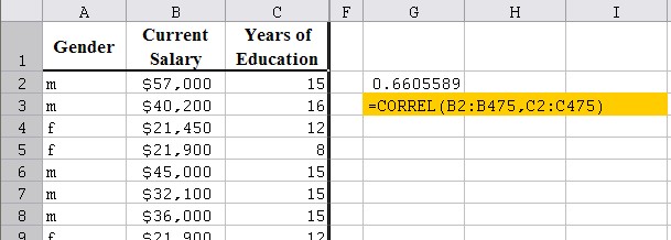
Since the correlation coefficient is 0.66 it means that there is indeed some positive relation between years of schooling and salary earnings. But since the value is not that close to +1.0, the relationship is not strong.
In the next sections we will introduce a more detailed analysis, which will allow us to not only to determine whether or not there is a linear relation, but also to compute the exact equation of that linear relation, which we can in turn use to make predictions. So, I hope that motivates you enough to read on.