 MathCS.org - Statistics
back | next
7.1 The Normal Distribution and its Relatives
We will now switch gears and start involving probabilities in our next discussions. This course is a course in Statistics, and not in Probability Theory, however, so we will only use as much probability as necessary to discuss statistical concepts, and we will not study probability theory in it's own right here. We will also, for the most part, restrict our attention to numerical variables only from now on.
First, let's briefly introduce the concept of probability and see how it relates to our previous work.
Probability: We will consider a "probability of an event" as the chance, or likelihood that an event indeed takes place. All probabilities will be numbers between 0.0 and 1.0, where a probability of 0 means that an event does not happen and a probability of 1.0 means that an event will happen for certain. We will often use the notation P(A) to denote the "probability of A". The total probability of all events must add up to 1.0.
Example: What is the probability in tossing one (fair) coin that it shows Heads. What is the probability in getting a number 5 or larger when throwing one die? What is the probability of two dice adding to 4 when tossing them simultaneously?
In many cases probabilities can be obtained by counting. In tossing a coin, for example, there are two possible outcomes, head and tail, and both are equally likely (if the coin is fair). Thus, the probability of obtaining a head outcome should be 1 out of 2, or 1/2, which in math simply means "1 divided by 2". Thus:
P(one Head) = 0.5
Similarly, for a die there are 6 possible outcomes, all equally likely. Thus, the event of obtaining a number 5 or more is comprised of the event of getting a 5 or a 6. Thus, the corresponding probability should be 2 out of 6, or 2/6, or 1/3.
P(5 or 6) = 1/3 = 0.3333
Finally, if we through two dice simultaenously, each could show a number from 1 to 6. To illustrate what happens, we create a table where each entry inside the table denotes the sum of the two dices:
1 2 3 4 5 6 1 2 3 4 5 6 7 2 3 4 5 6 7 8 3 4 5 6 7 8 9 4 5 6 7 8 9 10 5 6 7 8 9 10 11 6 7 8 9 10 11 12
But now it's again an exercise in counting: there are a total of 36 possible outcome. We are interested in the sum of the dice being 4, and from the table we see that there are 3 possible throws adding up to 4 (a 3+1, 2+2, and 1+3). Thus, our probability is 3 out of 36, or 3/36, which reduces to 1/12. Thus:
P(sum of two dices = 4) = 1/12 = 0.0833
Sample exercises: to see if you can compute probabilities by
counting, find (a) the probability of obtaining at least one tail
when tossing one coin twice, (c) the probability of getting a
Queen when randomly drawing
one card from a standard deck of 52 cards, and (c) the probability
of the sum being at most 10 when throwing two dice.
In more real-life experiments it may be too time consuming, or simply not possible, to list all possible outcomes to count out the ones we are interested in, but we can instead use a frequency histogram to come up with approximate probabilities. For example, suppose that a (hypothetical) frequency distribution for the age of people in a survey is as follows:
Here we simply used decimal numbers instead of percentages, i.e. the entry in the first row means that 15% of the people in the survey were between 0 and 18 years old.
Category Probability 0 – 18 0.15 19-40 0.25 41-65 65 and older 0.3
- One number is missing in the table above – what is that number?
- We know that probabilities have to add up to 1.0, so the missing number is 1.0 - (0.15 + 0.25 + 0.3) = 0.3. This works if one number is missing, but as soon as two numbers were missing this trick would no longer work.
- What is the chance that a randomly selected person is 40 years or younger?
- The event of being 40 years or younger means that a person is either in the 0 to 18 category, with probability 0.15, or in the 19 to 40 category, with probability 0.25. Therefore, the total probability or a person being younger than 40 is 0.15 + 0.25 = 0.40, or equivalently 40%.
Example: In section 5.2 we discussed a survey that asked 474 randomly selected people for their income level. If we were to meet one of these employees at random, what is the probability that this person has an annual income between $30,000 and $40,000?
If we followed the above example of coins and dice, we could simply count how many employees of the 474 participants earn between $30K and $40K. That number, out of 474, would be our desired probability. However, in section 5.2 we have already created frequency charts using percentages, and that chart can directly give us the answer. In our case, recall that the chart we created was:
From the chart we see that 22.57% of the people questioned earn between $30K and $40K, thus
P(annual salary between $30K and $40K) = 0.2557
In addition to a percentage chart it is often helpful to consider probabilities in relation to frequency histograms graphically.
Example: Consider the Excel Data set health_female.xls, showing a number of variables related to the health records of 40 female patients, randomly selected. Construct a frequency histogram for the height of the 40 patients, including a chart. Then use that histogram to find the following probabilities. For each question, shade the part of the histogram chart that you used to answer the question.
- What is the probability, approximately, that a woman is 60 inches or
- What is the probability, approximately, that a woman is 65 inches or
- What is the probability, approximately, that a woman is between 60 and 65 inches tall?
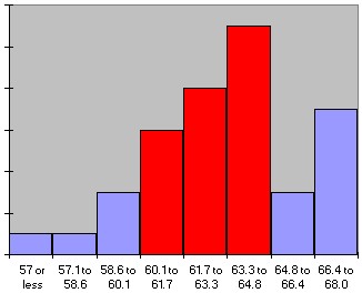
We first download the data set, as usual, and construct a frequency histogram (as discussed in section 3.4). We have chosen the specific bin boundaries as show in the picture, and we have modified the histogram table slightly to clarify the bin boundaries. We also computed the relative frequency for each row, defined as the number in that row divided by the total number of observations. The resulting table and chart look as follows:
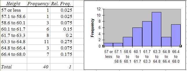
From this chart it is now easy to answer the questions. Note that our bin boundaries do not exactly correspond to the boundaries posed in the questions, but we can use the closest bin boundary available to get the approximately right answer.
- P(a woman is 60 inches or smaller) = (1 + 1 + 3) / 40 = 5 / 40 = (0.025 + 0.025 + 0.075) = 0.125 (or 12.5%)
- P(a woman is 65 inches or taller) = (3 + 7) / 40 = (0.075 + 0.175) = 0.25 (or 25.0 %)
- P(a woman is between 60 and 65 inches tall) = (6 + 8 + 11) / 40 = 25 / 40 = (0.15 + 0.2 + 0.275) = 0.625 (or 62.5%)
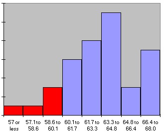
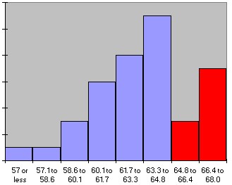
Graphically speaking (I know, you can't speak graphically -:) we have used the parts of the histogram shaded in red to compute the respective probabilities:
P(size <= 60) = 0.125
P(size >= 65) = 0.25
P(60 <= size <= 65) = 0.625
To make sure, our probabilities are approximate because the bin boundaries don't exactly match the questions. In addition, we have not really computed, for example, that the probability of "a woman" to be between 60 and 65 inches tall is 62.5%. Strictly speaking we have computed that the probability of a randomly selected woman out of our sample of 40 woman is between 60 and 65 inches tall is 62.5%.
But if in turn the entire sample was truly randomly selected, then it is a fair guess to say that:
the probability of any woman to be between 60 and 65 inches tall is 62.5%
where we have generalized from the woman in our sample to the set of all woman. It should be clear that the 62.5% answer is correct if all we consider is our 40 woman in the sample. It should be equally clear that this 62.5% is only approximately correct if we generalize to all woman.
In the next section we will clarify what we mean by approximately correct and we will introduce formulas to compute the error involved in this type of generalization. But before we can do that, we must discuss the concept of a Normal Distribution.
The Normal Distribution
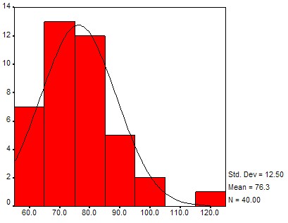
If you compute a lot of frequency histograms and their associated charts you might notice that most of them differ in detail but have somewhat similar shapes: the chart is "small" on the left and right side, with a "bump" in the middle. With a little bit of imagination you might say that many distributions look somewhat similar to a "church bell". Here are a few histogram charts, with the imagined "church bell" super-imposed (all of the data comes from the health_female.xls data file and a similar health_male.xls data file):
Height distribution
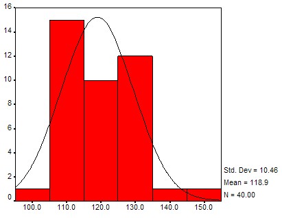
Pulse distribution
Systolic pressure distribution
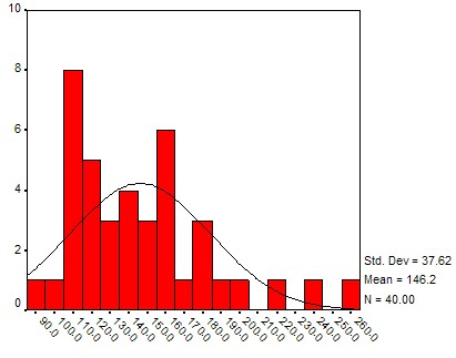
Weight distribution

These bell-shaped distributions differ from each other by the location of their hump and the width of bell's opening, and they have a special name:
Normal Distribution: A distribution that looks bell-shaped is called a normal distribution. The position of the hump is denoted by m and stands for the mean of the distribution, and the width is denoted by s and corresponds to the standard deviation. Thus, a particular normal distribution with mean m and standard deviation s is denoted by N(m, s). The special distribution N(0, 1) is called the standard Normal distribution.
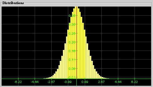
Standard Normal distribution N(0, 1)
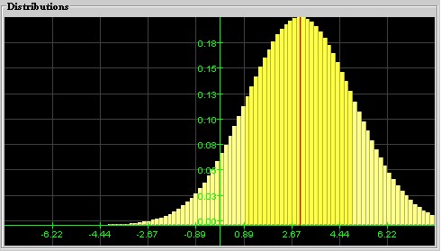
with mean 0 and standard deviation 1A Normal distribution N(3, 2) with mean 3
and standard deviation 2
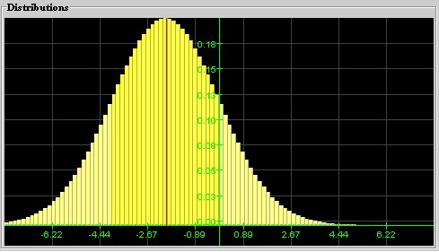
A Normal distribution N(-2, 3) with mean -2
and standard deviation 2
We can now use these normal distributions to help us compute probabilities.
Using Normal Distributions to Compute Probabilities with Excel
Instead of creating a frequency histogram with (more or less) arbitrary bin boundaries, compute the mean and the standard deviation of the data. Then use the normal distribution with that particular mean and standard deviation to compute the probabilities you are interested in.
Example: Before we considered the Excel Data set health_female.xls, showing a number of variables related to the health records of 40 female patients, randomly selected. Compute the mean and standard distribution for the height variable of that data set, then use the corresponding normal distribution to compute the probabilities below. For each question, shade the part of the normal distribution that you use to answer the question.
- What is the probability, approximately, that a woman is 60 inches or smaller?
- What is the probability, approximately, that a woman is 65 inches or taller?
- What is the probability, approximately, that a woman is between 60 and 65 inches tall?
As explained in chapter 4, we can use Excel to quickly compute the mean and standard deviation to be:
mean = 63.2, standard deviation = 2.74
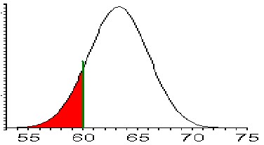
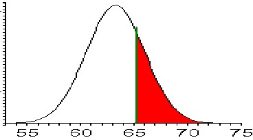
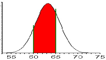
The corresponding normal distribution and the areas we have to figure out are pictured as follows:
To compute P(height <= 60)
we need to find the areaTo compute P(height >= 65)
we need to find the area:For P(60 <= height <= 65)
we need to find the area:
The good news is that Excel can easily compute these areas under a Normal Distribution. The bad news is that it is not completely straight-forward. Excel provides the formula:
NORMDIST(x, m, s, true)
where m and s are the mean and standard deviation, respectively, and the last parameter, at least for our purposes should be set to true. The value of that formula represents always the probability (aka area under the curve) from the left side under the normal distribution up to the value of x. For example:
| Excel formula | Math notation | Computed area | Actual Value |
| NORMDIST(0, 0, 1, true) | P(x <= 0), standard normal N(0, 1) |
 |
0.5 |
| NORMDIST(4, 2, 3, true) | P(x <= 4), normal N(2, 3) |
 |
0.7475 |
| NORMDIST(60, 63.2, 2.74, true) | P(x <= 60), normal N(63.2, 2.74) |
 |
0.1214 |
Note that the last value happens to be exactly the area we need to answer the first of our questions. Therefore:
P(x <= 60) = 0.1214
while the original method, using the actual frequency histogram, yields 0.125. Both computed values are close to each other, but using the Normal distribution is faster and allows for arbitrary boundary points to be used.
Other probabilities can be computed in a similar way, using the additional fact that the probability of everything must be 1. For example, suppose we want to use a N(63.2, 2.74) normal distribution to compute the probability P(height >= 65). If we simply used the Excel formula
NORMDIST(65, 63.2, 2.74)
then we would compute P(height <= 65), which is not what we want (in fact, it is kind of the opposite of what we want). However, it is clear that:
P(height <= 65) + P(height >= 65) = 1
because one of those two events must happen for sure. Therefore:
P(height >= 65) = 1 - P(height <= 65)
or shown as a picture
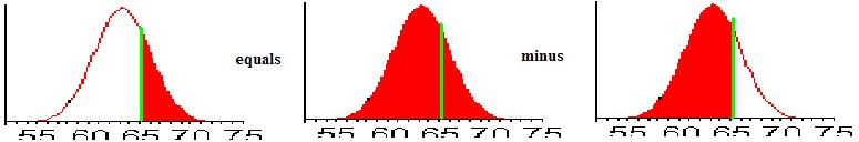
because of the way the NORMDIST Excel function is defined. To compute a probability like P(60 <= height <= 65), we can apply a similar trick:
P(60 <= height <= 65) = P(height <= 65) - P(height <= 60)
or shown as a picture
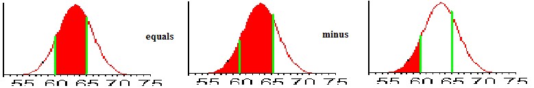
But now the important thing is to realize that in the right side the probabilities are computed for shaded areas that start on the left side of the distribution and go up to a specific value. That is exactly what the Excel formula NORMDIST computes, so we can now - finally - compute the probabilities in our question, using Excel:

Please note that there is a very close match between these probabilities and the probabilities computed using the actual frequency histogram.
Now, in fact, we can use Excel to rapidly compute probabilities without ever constructing a frequency histogram at all. In fact, we don't even need to have access to the complete data set, all we need is to know the mean and the standard deviation of my data so we can pick the right normal distribution to compute the probabilities.
Example: Consider the Excel Data set health_male.xls, showing a number of variables related to the health records of 40 male patients, randomly selected. Without constructing a frequency histogram for the height of the 40 patients, find the following probabilities:
- What is the probability, approximately, that a man is 60 inches or smaller?
- What is the probability, approximately, that a man is 65 inches or taller?
- What is the probability, approximately, that a man is between 60 and 65 inches tall?
Instead of constructing a complete frequency histogram, we quickly use Excel to compute the mean and the standard deviation of our data. Then we use the NORMDIST function, just as above, but of course using the mean and standard deviation for this data set, not the one we previously used. Here is a look at the Excel spreadsheet that shows the answer.
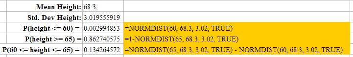
Note that the probability of a man being less than 60 inches tall is now about 0.003, or 0.3%, much lower than the probability for a woman. That makes sense, since men are, on average, taller than woman (68.3 inches versus 63.2 inches) so the probability of a man being less than 60 inches tall should indeed be lower than the comparable probability for women. The other figures equally make sense.
The computed probabilities will be (approximately) correct under the assumption that the height of men is indeed normally distributed, approximately.
Now it should be clear how to use the various normal distribution to quickly compute probabilities. To practice, here are a few exercises for you to do. The answers are listed, but not how to get them. Remember, you often can not use NORMDIST directly, you sometimes need to use 1 - NORMDIST or subtract two NORMDIST values from each other to get the correct answer. If you have any questions, please post them in our discussion area.
Example: Find the indicated probabilities, assuming that the variable x has a distribution with the given mean and standard deviation.
- x has mean 2.0 and standard deviation 1.0. Find P(x <= 3.0)
- x has mean 1.0 and standard deviation 2.0. Find P(x >= 1.5)
- x has mean -10 and standard deviation 5.0. Find P(-12 <= x <= -7)
- x is a standard normal variable. Find P(x <= -0.5)
- x is a standard normal variable. Find P(x >= -0.5)
- x is a standard normal variable. Find P(x >= 0.6)
- x is a standard normal variable. Find P(-0.3 <= x <= 0.4)
Answers:
- P(x <= 3.0) = 0.841344746
- P(x >= 1.5) = 0.401293674
- P(-12 <= x <= -7) = 0.381168624
- P(x <= -0.5) = 0.308537539
- P(x >= -0.5) = 0.691462461
- P(x >= 0.6) = 0.274253118
- P(-0.3 <= x <= 0.4) = 0.273333164