 MathCS.org - Statistics
8.2 Statistical Test for Population Mean (Large Sample)
In this section will try to answer the following question: It has been known that some population mean is, say, 10, but we suspect that the population mean for a population that has "undergone some treatment" is different from 10, perhaps larger than 10. We want to determine whether our suspicion is true or not.We will follow the outline of a statistical test as described in
the previous section, but adjust the four elements of the test to
our situation of testing for a population mean (we will see other
tests in subsequent sections).
At this stage we can setup the two competing hypothesis:
- Null Hypothesis H0: population mean = 10.0
- Alt. Hypothesis Ha: population mean not equal to 10.0
Since the sample mean is 11.3, which is more than other drugs, it looks like this sample mean supports our suspicion (because the mean from our sample is indeed bigger than 10). But - knowing that we can never be 100% certain - we must compute a probability and associate that with our conclusion.
Assuming that the null hypothesis is true we will try to
compute the probability that a particular sample mean (such as the
one we collected) could indeed occur. Leaving the details of the
computation aside for now, it turns out that the associated
probability
p = 0.044But if that computation is correct (which it is -:) we have a problem: assuming that the null hypothesis is true, the probability of observing a random sample mean of 11.3 or more is quite small (less than 5%). But we have observed a sample mean of 11.3, there no denying that fact. So, something is not right: either we were extremely lucky to have hit the less than 5% case, or something else is wrong: our assumption that the null hypothesis was true. Since we don't believe in luck, we choose to reject the null hypothesis (even though there's a 4.4% chance - based on our evidence - that the null hypothesis could still be right).
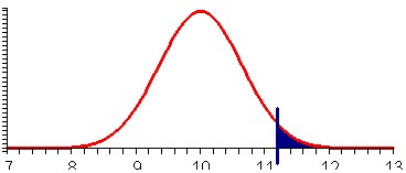
We want to know the chance that a sample mean could be 11.3 (or more), given that we assume the population mean to be 10.0 (our null hypothesis). In other words, we want to compute:
But from chapter 7.2 (Central Limit Theorem) we do know the distribution of sample means: according to that theorem we know that the mean of the sample means is the same as the population mean, and the standard deviation is the original standard deviation divided by the square root of N (the sample size). In other words, if the original mean is m and the original standard deviation is s, then the distribution of the sample means are N(m, s / sqrt(n) ). And since we assumed the null hypothesis was true, we actually know (as per assumption) the population mean, and - since nothing else is available, we use the standard deviation as computed from the sample to figure as the standard deviation we need. Therefore, we know that, in our case:
mean to use: 10.0But now Excel can, of course, help perfectly fine: it provides the function called "NORMDIST" to compute probabilies such as this one.Therefore, using the Central Limit Theorem:
standard deviation to use: 5.1/sqrt(62)
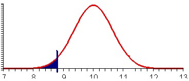
But we are not yet done: right now we only took into account that the sample mean could be 11.3 = 10 + 1.3 or more, whereas our alternative was that the mean is not equal to 10.0. Therefore we should also take into account that the probability could be smaller than 10 - 1.3 = 8.7. Again, Excel let's us compute this easily:
Finally, since the alternative hypothesis is not equal to 10.0 we need to consider both probabilities together. In other words, the value of p we need is, using symmetry of the normal distribution:
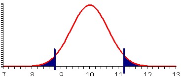
p = P(sample mean < 8.7) + P(sample mean > 11.3) = 2 * (1 - NORMDIST(11.3, 10.0, 5.1/sqrt(62), TRUE)) = 0.044
In chapter 7.1 we learned how to use the NORMDIST function to compute probabilities such as the ones we are interested in, but NORMDIST is somewhat difficult to use (we have to enter all these parameters at the right place). To simplify our calculation, we will instead use the new Excel function
which gives the probability using a standard normal distribution (mean 0, standard deviation 1), instead of the usual NORMDIST(x, m, s, TRUE) function. It is simpler to use because it requires only one input value. Both functions are related as follows:
Therefore, to compute probabilities we now proceed in two steps:
- Step 1: compute the
so-called z-score
z = (x - m) / ( s / sqrt(n) )
(notice the extra set of
parenthesis around numerator and denominator)
- Step 2: compute the probability using NORMSDIST(z) instead of NORMDIST(x, m, s/sqrt(n), TRUE)
- z = (11.3 - 10) / (5.1 / sqrt(62)) = 1.71, or in Excel, use:
= (11.3 - 10) / (5.1 / sqrt(62)) - p = 2 * (1 - NORMSDIST(2.01)) = 0.44, or in Excel use:
= 2 * (1 - NORMSDIST(2.01)
In other words, instead of entering the original mean, standard deviation, and sample size into the NORMDIST function we first compute a z-score, and then we use the NORMSDIST function to compute a probability.
Now we are ready to summarize our example into a procedure for testing for a sample mean as follows. The good news is that even if the above derivation seems complicated and perhaps confusing, the procedure we will now summarize is relatively simple and straight-forward. It works fine even if you did not understand the above calculations, as the subsequent examples will illustrate.
Statistical Test for the Mean (large sample size N > 30):
Fix an error level you are comfortable with (something like 10%, 5%, or 1% is most common). Denote that "comfortable error level" by the letter "A" If no prescribed comfort level A is given, use 0.05 as a default value. Then setup the test as follows:
- Null Hypothesis H0:
- mean = M, i.e. The mean is a known number M
- Alternative Hypothesis Ha:
- mean ≠ M, i.e. mean is different from M (2-tail test)
- Test Statistics:
- Select a random sample of size N, compute its sample mean X and the standard deviation S. Then compute the corresponding z-score as follows:
Z = (X - M) / ( S / sqrt(N) )- Rejection Region (Conclusion)
Compute p = 2*P(z > |Z|) = 2 * (1 - NORMSDIST(ABS(Z)))
If the probability p computed in the above step is less than A (the error level you were comfortable with initially, you reject the null hypothesis H0 and accept the alternative hypothesis. Otherwise you declare your test inconclusive.
Comments
- The null hypothesis, for this test, is that the population mean is always equal to a particular number. That number is usually thought of as the "default value", or the "status quo", or the "best guess" value. It is usually mentioned somewhere in the problem.
- The alternative hypothesis could actually be split into 3 possibilities (mean less than M, mean greater than M, or mean not equal to M). However, for simplicity we will restrict ourselves to the more conservative case where mean is not equal to M. Note that this is called a "2-tailed" test, while "mean < M" or "mean > M" would be called "1-tailed" test - we only consider 2-tailed tests.
- After computing the z-score in the third step you use the
NORMSDIST function, not
the NORMDIST function, to compute your probability in the last
step. Note that the ABS function mentioned in the above recipe
stands for "absolute value".
- Your conclusion is always one of two options: you
either reject the null hypothesis or declare your test
invalid. You never conclude anything else, such as
accepting the null hypothesis. If the comfort level A is not
given in a particular problem, use 5%, or A = 0.05.
- The standard deviations of the sample and the population are the same and are known
- The sample size is 30 or more
- Reject the null hypothesis when in fact it is true (Type I - Error). That's exactly the error we are computing in the procedure above as "level of significance".
- Accept the null hypothesis when in fact it is false (Type II - Error). This type of probability is not covered by our procedure (which is why we neve accept the null hypothesis, we rather declare our test inconclusive if necessary
Example 2: Bottles of ketchup are filled automatically
by a machine which must be adjusted periodically to increase or
decrease the average content per bottle. Each bottle is supposed to
contain 18 oz. It is important to detect an average content
significantly above or below 18 oz so that the machine can be
adjuste:; too much ketchup per bottle would be unprofitable, while
too little would be a poor business practice and open the company up
to law suites about invalid labeling.
We select a random sample of 32 bottles filled by the machine and compute their average weight to be 18.34 with a standard deviation of 0.7334. Should we adjust the machine? Use a comfort level of 5%.
We can see right away that the average weight of our sample, being 18.34 oz, is indeed different from what it's supposed to be (18 oz), but the question is whether the difference is statistically significant. In our particular case we want to know whether the machine is "off" and be sure to allow at most a 5% chance of an error in our conclusion. After all, if we did conclude the difference is significant we would have to adjust the Ketchup machine, which is an expensive procedure that we don't want to perform unnecessarily.
Our statistical test for the mean will provide the answer:
- The Null Hypothesis is: the mean is equal to 18, i.e. "everything is fine"
- The Alternative Hypothesis is: mean is not equal to 18 (2-tail test), i.e. we should adjust the machine
- The Test Statistics: sample mean is 18.34, standard
deviation is 0.7334, sample size is 32. Compute the z-score as
follows
Z = (18.34 - 18) / (0.7334 / sqrt(32)) = 2.622
- We use Excel to compute p = 2*(1-NORMSDIST(2.622)) = 0.0087, according to case (c) of our procedure. That probability is smaller than our comfort level A = 0.05 (or 5%) so that we reject the null hypothesis
Example 3: In a nutrition study, 48 calves were fed
"factor X" exclusively for six weeks. The weight gain was recorded
for each calf, yielding a sample mean of 22.4 pounds and a standard
deviation of 11.5 pounds. Other nutritional supplements are known to
cause an average weight gain of about 20 lb in six weeks. Can we
conclude from this evidence that, in general, a six-week diet of
"factor X" will yield an average weight gain of 20 pounds or more at
the "1% level of significance"? In other words, is "factor X"
significantly better than standard supplements?
- The Null Hypothesis is: the mean is equal to 20, i.e. there is no improvement, everything is as it's always been
- The Alternative Hypothesis is: the mean is not equal 20 (we actually want to know whether "factor X" results in higher average weight gains, which would be a 1-tail test but for simplicity we change the alt. hypothesis to check simply for a difference in weight gain)
- Test statistics:
sample mean is 22.4, standard deviation is 11.5, sample size is
48. Compute the z-score
Z= (22.4 - 20) / (11.5 / sqrt(48) ) = 1.446
- We use Excel to compute p = 2*(1 - NORMSDIST(1.446)) = 0.148, or 14.8%. This probability is relatively large: if we rejected the null hypothesis, the probability that we made a mistake is 14.8%. That is larger than our comfort level of 1%, so our conclusion is: the test is inconclusive
Example 4: A group of secondary education student teachers were given 2 1/2 days of training in interpersonal communication group work. The effect of such a training session on the dogmatic nature of the student teachers was measured y the difference of scores on the "Rokeach Dogmatism test given before and after the training session. The difference "post minus pre score" was recorded as follows:
-16, -5, 4, 19, -40, -16, -29, 15, -2, 0, 5, -23, -3, 16, -8, 9, -14, -33, -64, -33Can we conclude from this evidence that the training session makes student teachers less dogmatic (at the 5% level of significance) ?
We can easily compute (using Excel) that the sample mean is -10.9 and the standard deviation is 21.33. The sample size N = 20. Our hypothesis testing procedure is as follows:
- Null Hypothesis: there is no difference in dogmatism, i.e. mean = 0
- Alternative Hypothesis: there is a difference in dogmatism, i.e. mean not equal to 0 (note that we again switched from a 1-tail test - dogmatism actually goes down - to a 2-tail test - dogmatism is different, for simplicity).
- Test statistics:
sample mean = -10.9, standard deviation = 21.33, sample size =
20. Compute the z score:
z = (-10.9 - 0) / (21.33 / sqrt(20) ) = -2.28
- We use Excel to compute p = 2*(1 - NORMSDIST(2.28)) = 0.022, or 2.2%. That probability is less than 0.05 so we reject the null hypothesis
Thus, since we reject the null hypothesis we accept the alternative, or in other words we do believe that the training session makes the student teachers differently dogmatic, and since the mean did go down, less dogmatic. The probability that this is incorrect is less than 5% (or about 2.2% to be precise). For curious minds: for the 1-tail test p would have worked out to be p = 1.1% (half the 2-tail value) which would also have lead to a rejection of the null hypothesis at the 5% level.
Please note that technically we were not supposed to use our procedure, since the sample size N = 20 is less than 30. Therefore, while we can still reject the null hypothesis, the true error in making that statement is somewhat larger than 2.2%. So, you ask: "what are we supposed to do for small sample sizes N < 30"? Funny you should ask - there's always another section ...